Here in this article we shall see how to solve unforced LTI differential equations and meet the characteristic equation and handle multiple and complex roots of the characteristic equation.
Also, see how to determine the constants that arise in the solution of the differential equations. When given the initial conditions, this amounts to solving a set of equations. For circuit problems, where the initial conditions are given in terms of circuit values, the initial conditions of the function must first be found, then the constants must be found.
We know that differential equations can be used to represent a circuit response. We are interested in finding solutions of the differential equations, because the solution represents what the system is doing. We will begin by looking at the differential equation in the traditional way, from the “time domain”. Later we will cover other very elegant methods of solving the equations using Laplace transforms.
Differential equations:
Mathematicians usually treat the solution of differential equations by finding the homogeneous solution and the forced solution. We often break the solution into the “zero-input” response and the “zero-state” response.
Zero-input response The response of the system when there is no input forcing function. The output resulting is due to initial conditions of the system. (For example, charge on a capacitor.)
Zero-state response When a system is in zero-state, it is assumed that the initial conditions are all zero (the “zero state”). Thus, the response of the system is due to some kind of external input.
The output is the sum of the zero-input response and the zero-state response, because we are dealing with linear systems:
Total response = zero-input response + zero-state response.
In general, a LTIC (linear, time-invariant, continuous time) can be expressed in terms of differential equation
In operator notation
Let
Then
Usually we will have m ≤ n.
Let y0(t) be the zero-input response, i.e., the response when f(t) = 0. Let yz-s(t) be the zero-state response, when f(t) ≠0 but the initial conditions are zero.
Let us start with yz-i(t). That is, the input f(t) is assumed to be zero, so we have
or
(y0(t) is what the book uses as the zero-input response.) Take a simple example: (RL circuit)
This is the key equation: the derivative of the solution has the same form as the solution.
Integrate:
Observe that in general if
that
So all we have to do is to match coefficients.
What is C? We must have some extra information to tell us - some specific value of the solution at some time. This is often the initial condition. We must know, for example, the initial current on the inductor. (Plot some examples.) If y0(0) is known, then we have
More generally, take Q(D)y0(t) = 0, or
Assume a solution of the form
for some c and some λ, to be determined. Substituting (expand the derivatives) we get
which could be written as
There are two possible ways this could happen: either c = 0, would be the case if there is no zero-input response (all the initial conditions are zero); or
Note that this is a polynomial in λ of degree n. It has n solutions, which we will write as λ1, λ2, . . . ., λn. That is,
how do we find the roots? If it is quadratic equation, you can do it yourself, lickety split. Anything higher, plan to use a computer (that's why they were invented!). Use Matlab, for example.
So let
Take them all | this is, after all, a linear system. The sum of any solutions is another solution. So we will take
This provides the total solution, provided that we can find all of the constants c1, c2, . . . . , cn.
Recap: Assume solution, substitute in the DE, then find roots to equation and combine together. Don't lose sight of the fact that there is a physical system behind all this.
The equation
is called the characteristic equation. Recall from the example we did on linear algebra that we have the same denominator in all solutions. It turns out that this denominator is also the characteristic equation.
The overall system behavior of the system is determined by the characteristic equation. The values of that are the roots are known as the modes or natural frequencies or eigenmodes or eigenvalues or characteristic values of the system.
Example 1
A simple 2nd-order system

Assume we have initial conditions

Example 2
A 2nd-order system with complex roots:

This is a little yucky. Let us suppose that the constants are complex conjugates:
Then y0(t) is real. Then (work through)
Observe: damping comes from real part; frequency comes from imaginary part. Plot poles on complex plane, and discuss placement.
This example with complex roots is true in general. If we have a 2nd order system so that
that is real, then c1 and c2 must be conjugates; let
Then
Discuss. Plot some pole locations and discuss. Stability...
Example 3
Repeated roots. Things become somewhat more complicated when the characteristic equation has repeated roots. For example, suppose
In this case, let
This satisfies the DE. (Homework: show this!).
In the general case, if there is a repeated root
then
satisfies the DE. If there is a repeated root
then
satisfies the DE. The corresponding characteristic modes are eλt, teλt, . . . . ., tr-1eλt.
Solving for the parameters
Whenever we do a differentiation in mathematics, some information is lost. For example, if we take the derivative of a position variable, we obtain the velocity, but not the position. If we integrate the velocity, we must have some information in order to regain the position. For example, if y(t) is the position, and we know that
then the best we can say is
We do not know the position. However, if we knew the position at some time t0, we could use this:

Such information is always required in solving differential equations. Usually it is given in the form of initial conditions.
Example 4
Circuit. vC(0) = 5, y(0) = 0.
We have
Need to derive initial condition (of y) from initial conditions of the circuit. Remove voltage source (since nding y0(t)). Initial condition on inductor → y0(0) = 0. Now write loop equation (w/o source):

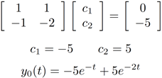
Then (substituting in the solution)

For these equations, it is always possible to put them in a matrix form. (The exception is for complex roots, when some trig usually becomes involved.) Write as

As you work with larger DEs, being able to express in matrix form and using a matrix tool will be beneficial to you.
In the general case, with n DEs you will need n initial conditions to obtain the solution unambiguously.
Recap:
- Write the differential equation for the system.
- For the zero-input solution, assume that the source(s) are zero.
- Find the solution for the differential equation with variables for the amplitudes of each of the modes.
- Solve for the initial conditions of the equation from the initial conditions of the circuit (requires going back to the circuit analysis usually).
- Using these initial conditions, solve for the variables in the solution.
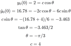
Example 5
with initial conditions
At t = 0:

I have doubt in Example 5. The way it is solved has confused me .please explain me .
ReplyDelete