previous MODELING A STABELIZATION FIXTURE WITH END PRESSURE USING SOLID ELEMENTS
The beam below is cantilevered or "built in" on the left edge. This means that both the translations and the rotations are held to zero along this edge. The material properties for the beam are E= 70 x 109 Pascals (typical for Aluminum) and n = 0.3 . The beam has a solid rectangular cross section with thickness in the Z-direction t = 0.01 meters and height in the Y-direction h = 0.1 meters. We wish to find the mode shapes and associated vibration frequencies for this beam.

Assume the element has the configuration shown below:
Our goal is to find the element stiffness matrix

ASSUME: 2 displacement degrees of freedom (dof) per node With :
[B] = the strain - displacement matrix such that [B]{u} = {ε}
where: {u} is the dof vector and {ε} is the strain vector
[E] = the constitutive matrix such that [E]{ε} = {σ}
where {σ} is the stress vector and V = volume.
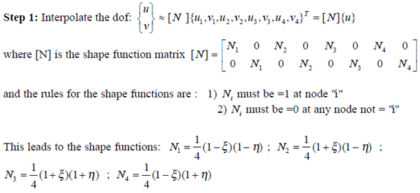
Step 2: Find the [B] matrix:
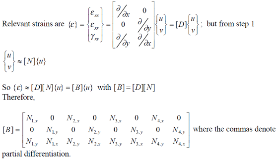
Step 3: Use the Jacobian to find derivatives:


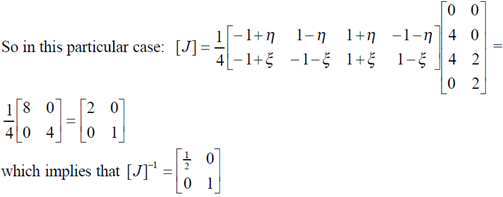
This allows us to find the entries in [B]
Step 4: Perform the numerical integration:

where |J| is the determinant of the Jacobian matrix.

The elements as formed above must be assembled into a global stiffness matrix. In the same manner, element mass matrices are formed using the equation
a) Log on to the computer
b) Click START (lower left corner of the Windows Desktop), go to Programs, Select MSC (common), Select MSC Patran9.0.
Click = Unless otherwise stated, this indicates a click with the left mouse button.
Boldface will indicate text that occurs in the PATRAN menus.
Italics text will indicate text that you must enter into text boxes in the PATRAN menus or text that you choose in a menu scroll box.
1. Our first step is to create a new database:
From the TM choose File In the resulting pull down menu choose New
A SM called New Database pops up
Turn on (checked) Modify Preferences Under File Name enter beam-vib.db
Click OK
2. Next set the analysis preference:
A New Model Preferences window will appear as a RM
Under Tolerance choose Based on Model
Set Model Dimension to10.0
Under Analysis Code choose MSC/NASTRAN
Choose Analysis Type = Structural
click OK
3. The geometry of the beam will be determined next: From the TM choose Geometry A RM called Geometry will result
Set Action = Create
Object = Point
Method = XYZ
Set the Point ID list to 1
Set Reference Coordinate Frame to Coord 0
Turn off the Auto Execute button
Enter the following into the Point Coordinates list:
[0,0,0] (note that PATRAN will accept either commas or blanks as separators between coordinates)
Click Apply
A point will appear in the main viewport at coordinates [0,0,0]
Use this same procedure to create points at coordinates [1,0,0], [1,0.1,0] and [0,0.1,0]
Back at the top of the RM called Geometry
Set Action = Create
Object = Curve
Method = Point Set the Curve ID list to 1
Turn Autoexecute off
Set Starting Point List = Point 1
Set Ending Point List = Point 2
Click Apply
Back at the top of the RM called Geometry
Set Action = Create
Object = Curve
Method = Point
Set the Curve ID list to 2
Turn Autoexecute off
Set Starting Point List = Point 3 Set Ending Point List = Point 4
Click Apply
Back at the top of the RM called Geometry
Set Action = Create Object = Surface
Method = Curve
Set the Surface ID list to 1
Set Patran 2 Convention off Option = 2 Curve
Set Manifold off (not checked)
Set Starting Curve List = Curve 1 Set Ending Curve List = Curve 2
Click Apply
2. The finite element mesh is specified next:
From the TM choose Elements
A RM appears called Elements
Set Action = Create Object = Mesh
Type = Surface
Set Node Id = 1
Set Element Id List = 1 Set Global Edge Length = 0.025
Set Element Topology = Quad4
Set Mesher = Isomesh
Click in the Surface List box
Click and drag to select the entire structure
The Words "Surface 1" should appear in the Surface List Click Apply
From the TM choose Load/BC's A RM called Load/Boundary Conditions will appear
Set Action = Create
Object = Displacement
Type = Nodal
Set Current Load Case = Default Enter New Set Name as l_cant ( The name can be whatever name you wish. The name l_cant is chosen as this is for the cantilever of the left most nodes)
Click Input Data... a SM called Input Data appears
Set Load/BC Scale factor = 1
Set Translations to <0,0,0> Set Rotations to <0,0,0> Be sure Analysis Coordinate Frame is Coord0
Click OK
(back in the Load/Boundary Conditions RM)
Click Select Application Region A SM called Select Application Region appears
Turn on the FEM (button down)
Click in box under Select Nodes
Use the cursor to highlight the set of nodes along the left vertical edge of the beam. There should be 5 nodes there.
Click OK
(The Load / Boundary Condition RM appears again)
Click Apply
On the TM select Materials a RM will appear called Materials
Set Action = Create
Object = Isotropic
Method = Manual Input
Click Material Name box
Input the name to be aluminum Click Input Properties box
SM called Input Options appears
Input Elastic Modulus =70.0E9 Input Poisson = 0.3
Input the Density to be 2700
Click OK Back in the Materials RM
Click Apply
5. The properties for each element are assigned next: On the TM select Properties
a RM will appear called Element Properties
Set Action = Create Dimension = 2d
Type = Shell
Click Property Set Name box
Enter beam_prop
Click Input Properties
a SM appears called Input Properties
Click in the Material Name box
Click on the word "aluminum" in the Material Property Sets box at the bottom of the SM
( the words m:aluminum will appear in the Material Name box at the top of the SM)
Click in the Thickness box
Enter 0.01
Click OK
(Back in the Element Properties RM)
Click Select Members box
a Patran Select menu will appear on the left edge of the RM
Click on the icon which contains the surface or face icon
Click Add
(The words Surface 1 appears in the Application Region box)
Click Apply in the Element Properties menu
(beam_prop will be added to the Existing Property Sets box)
6. The analysis is to be done is specified next:
On the TM select Analysis
a RM will appear called Analysis Set Action = Analyze
Object = Entire Model
Method = Full Run
Click Translation Parameters
In the SM that appears, set Data Output = Op2 and Print Click OK Back in the RM Analysis Set Solution Type = Normal Modes (button down)
Click OK
Click Apply (The analysis will take a few seconds to run. A SM indicating that MSC/Nastran is working may appear)
A RM will appear called Results Set Action = Create
Object = Quick Plot
In the Select Result Case box click Default, Mode 1…
In the Select Fringe Result box click Eigenvectors, translational
In the Apply Fringe Result box click Eigenvectors, translational Set Quantity = Magnitude
Turn on the animation button (so it displays a check)
Click Apply (This will create the animation of the first mode)
On the TM select File
From the pull down menu select Save
On the TM select File From the pull down menu select Quit
next THERMAL ANALYSIS OF A COOLING FIN USING SHELL ELEMENTS
MSC/PATRAN TUTORIAL # 6
MODELING A CANTILEVERED BEAM’S VIBRATION USING 4 NODE SHELL ELEMENTS
I. THE PHYSICAL PROBLEM MODELING A CANTILEVERED BEAM’S VIBRATION USING 4 NODE SHELL ELEMENTS
The beam below is cantilevered or "built in" on the left edge. This means that both the translations and the rotations are held to zero along this edge. The material properties for the beam are E= 70 x 109 Pascals (typical for Aluminum) and n = 0.3 . The beam has a solid rectangular cross section with thickness in the Z-direction t = 0.01 meters and height in the Y-direction h = 0.1 meters. We wish to find the mode shapes and associated vibration frequencies for this beam.

II. THINKING ABOUT THE MECHANICS
The analytic solution (modes shapes and natural frequencies) for this problem is readily available. Any vibrations text will provide equations for the mode shapes (eigenvectors) and the natural frequencies (eigenvalues). These equations are given below. For the cantilevered beam with bending moment of inertia “I”, Elastic (Young’s) modulus “E”, mass per unit length “m” and Length “L”, the first 3 natural frequencies W1-3 (rad/sec) are given by:
The analytic solution (modes shapes and natural frequencies) for this problem is readily available. Any vibrations text will provide equations for the mode shapes (eigenvectors) and the natural frequencies (eigenvalues). These equations are given below. For the cantilevered beam with bending moment of inertia “I”, Elastic (Young’s) modulus “E”, mass per unit length “m” and Length “L”, the first 3 natural frequencies W1-3 (rad/sec) are given by:
Note that these correspond to the following 3 mode shapes which are all bending modes in the plane of the smallest value of “I”.
Modeshape 1:
Modeshape 2:
Modeshape 3:
Some basic questions to consider before creating the computational model are:- Are there any other types of mode shapes that might occur (torsional, axial or bending in a different plane)?
- What would be a reasonable frequency for the first mode shape?
- Are there any constraint force checks that will help me validate the accuracy of my model?
Answering these questions qualitatively, along with the quantitative analytical solutions for the mode shapes and their associated natural frequencies will provide reinforcement that your computational model is correctly constructed.
III. GEOMETRIC AND FINITE ELEMENT MODEL As is the standard procedure for building MSC/Patran models, we will build the geometry first and then construct a finite element mesh on that geometry. The geometry will proceed from creation of points to curves to surfaces for this simple model. Next, we will use 4 node shell elements to model the beam. Next, the material and element properties will be entered. We will constrain the 3 displacement and 3 rotational degrees of freedom on the left edge (for all nodes). This creates the cantilevered or built-in, end condition. Finally, the nodes must be equivalenced before the analysis is ready to run.
IV. FINITE ELEMENT THEORY The exact details of the formulation of the 4 node shell elements in MSC/Nastran is rather complicated. However, the basic formulation of an isoparametric 4 node membrane element is not extremely difficult and will provide us with sufficient background information to begin to understand the vibration model studies. This basic form is constructed as follows:
Isoparametric Formulation of a 2-D Membrane Element [K] Matrix Assume the element has the configuration shown below:
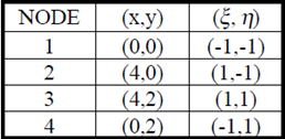
The physical and natural coordinate locations of the 4 nodes are:

Our goal is to find the element stiffness matrix
ASSUME: 2 displacement degrees of freedom (dof) per node With :
[B] = the strain - displacement matrix such that [B]{u} = {ε}
where: {u} is the dof vector and {ε} is the strain vector
[E] = the constitutive matrix such that [E]{ε} = {σ}
where {σ} is the stress vector and V = volume.

Step 2: Find the [B] matrix:

Step 3: Use the Jacobian to find derivatives:
i.e. the isoparametric assumption is that geometry can be interpolated using the same interpolation functions as the displacements.


This allows us to find the entries in [B]
Step 4: Perform the numerical integration:

where |J| is the determinant of the Jacobian matrix.
Gaussian numerical integration is then used to find the final numbers for the element stiffness.
Where ngj and ngi are the number of gaussian integration points in the “j” and “i” directions respectively and wj and wi are the associated gaussian weighting factors.
Understanding the Computational Vibration Analysis : The elements as formed above must be assembled into a global stiffness matrix. In the same manner, element mass matrices are formed using the equation
[M] = ρʃ[N]T [N] J dx dh . A similar form exists for the Rayleigh damping matrix  . A similar form exists for the Rayleigh damping matrix [C]. The stiffness, mass and damping matrices are then used in the dynamics equilibrium relationship
  where the over-dots indicated derivatives with respect to time and {f} is the forcing function. This set of equations can be solved for the time history of the motion (transient dynamics) or for the eigenvalues and eigenvectors. For the vibration analysis, the damping and the forcing function are assumed to be zero. The resulting eigenvalue problem of the second kind is : [M] {w} + [K] {d} = {0} where eigenvalues are the natural frequencies w and the eigenvectors {d} give the node shapes.
V. STEP BY STEP INSTRUCTIONS FOR MODELING THE VIBRATION OF THE CANTILEVERED BEAM USING MSC/PATRAN
Preliminaries for using PATRAN include: a) Log on to the computer
b) Click START (lower left corner of the Windows Desktop), go to Programs, Select MSC (common), Select MSC Patran9.0.
In the instructions below, the following abbreviations and terms will be used:
TM = Top Menu. This refers to the horizontal menu options residing at the top of the screen after PATRAN has been initiated.
TM = Top Menu. This refers to the horizontal menu options residing at the top of the screen after PATRAN has been initiated.
RM = Right Menu. This refers to the menus that pop up after an option has been chosen from the top menu. These menus reside on the far right side of the PATRAN desktop.
SM = Subordinate Menu. This referees to the menus that pop up from options selected in the right menu.Click = Unless otherwise stated, this indicates a click with the left mouse button.
Boldface will indicate text that occurs in the PATRAN menus.
Italics text will indicate text that you must enter into text boxes in the PATRAN menus or text that you choose in a menu scroll box.
1. Our first step is to create a new database:
From the TM choose File In the resulting pull down menu choose New
A SM called New Database pops up
Turn on (checked) Modify Preferences Under File Name enter beam-vib.db
Click OK
2. Next set the analysis preference:
A New Model Preferences window will appear as a RM
Under Tolerance choose Based on Model
Set Model Dimension to10.0
Under Analysis Code choose MSC/NASTRAN
Choose Analysis Type = Structural
click OK
3. The geometry of the beam will be determined next: From the TM choose Geometry A RM called Geometry will result
Set Action = Create
Object = Point
Method = XYZ
Set the Point ID list to 1
Set Reference Coordinate Frame to Coord 0
Turn off the Auto Execute button
Enter the following into the Point Coordinates list:
[0,0,0] (note that PATRAN will accept either commas or blanks as separators between coordinates)
Click Apply
A point will appear in the main viewport at coordinates [0,0,0]
Use this same procedure to create points at coordinates [1,0,0], [1,0.1,0] and [0,0.1,0]
Back at the top of the RM called Geometry
Set Action = Create
Object = Curve
Method = Point Set the Curve ID list to 1
Turn Autoexecute off
Set Starting Point List = Point 1
Set Ending Point List = Point 2
Click Apply
Back at the top of the RM called Geometry
Set Action = Create
Object = Curve
Method = Point
Set the Curve ID list to 2
Turn Autoexecute off
Set Starting Point List = Point 3 Set Ending Point List = Point 4
Click Apply
Back at the top of the RM called Geometry
Set Action = Create Object = Surface
Method = Curve
Set the Surface ID list to 1
Set Patran 2 Convention off Option = 2 Curve
Set Manifold off (not checked)
Set Starting Curve List = Curve 1 Set Ending Curve List = Curve 2
Click Apply
2. The finite element mesh is specified next:
From the TM choose Elements
A RM appears called Elements
Set Action = Create Object = Mesh
Type = Surface
Set Node Id = 1
Set Element Id List = 1 Set Global Edge Length = 0.025
Set Element Topology = Quad4
Set Mesher = Isomesh
Click in the Surface List box
Click and drag to select the entire structure
The Words "Surface 1" should appear in the Surface List Click Apply
Set Action = Equivalence
Object = All
Type = Tolerance Cube
(The purpose here is to tie the nodes together that lie on top of one another)
Set the Equivalencing Tolerance to .003
Click Apply (The command window at the bottom of the PATRAN desktop will tell you that 0 nodes were deleted. This step will become critical if, in more complicated models, you are attempting to join portions of a model which have been meshed separately.)
3. The boundary conditions are specified next: Object = All
Type = Tolerance Cube
(The purpose here is to tie the nodes together that lie on top of one another)
Set the Equivalencing Tolerance to .003
Click Apply (The command window at the bottom of the PATRAN desktop will tell you that 0 nodes were deleted. This step will become critical if, in more complicated models, you are attempting to join portions of a model which have been meshed separately.)
From the TM choose Load/BC's A RM called Load/Boundary Conditions will appear
Set Action = Create
Object = Displacement
Type = Nodal
Set Current Load Case = Default Enter New Set Name as l_cant ( The name can be whatever name you wish. The name l_cant is chosen as this is for the cantilever of the left most nodes)
Click Input Data... a SM called Input Data appears
Set Load/BC Scale factor = 1
Set Translations to <0,0,0> Set Rotations to <0,0,0> Be sure Analysis Coordinate Frame is Coord0
Click OK
(back in the Load/Boundary Conditions RM)
Click Select Application Region A SM called Select Application Region appears
Turn on the FEM (button down)
Click in box under Select Nodes
Use the cursor to highlight the set of nodes along the left vertical edge of the beam. There should be 5 nodes there.
Click OK
(The Load / Boundary Condition RM appears again)
Click Apply
(3 displacement constraint arrows and 3 rotation constraint arrows should now appear on each node in the main viewport window on the extreme left edge of the beam. Numbers 1,2,3,4,5,6 will appear with the arrows to show that all 6 of the dof are constrained there)
4. The materials are specified next: On the TM select Materials a RM will appear called Materials
Set Action = Create
Object = Isotropic
Method = Manual Input
Click Material Name box
Input the name to be aluminum Click Input Properties box
SM called Input Options appears
Input Elastic Modulus =70.0E9 Input Poisson = 0.3
Input the Density to be 2700
Click OK Back in the Materials RM
Click Apply
5. The properties for each element are assigned next: On the TM select Properties
a RM will appear called Element Properties
Set Action = Create Dimension = 2d
Type = Shell
Click Property Set Name box
Enter beam_prop
Click Input Properties
a SM appears called Input Properties
Click in the Material Name box
Click on the word "aluminum" in the Material Property Sets box at the bottom of the SM
( the words m:aluminum will appear in the Material Name box at the top of the SM)
Click in the Thickness box
Enter 0.01
Click OK
(Back in the Element Properties RM)
Click Select Members box
a Patran Select menu will appear on the left edge of the RM
Click on the icon which contains the surface or face icon
Move the cursor arrow to a point to the left and above the highest, leftmost point on the beam. Click and hold down the left mouse button. Drag the cursor (while holding down the mouse button) to a point to the right of and below the right-most bottom node. A "selection box" is formed while you drag. Release the button.
(The words Surface 1 will appear in the Select Members box) Click Add
(The words Surface 1 appears in the Application Region box)
Click Apply in the Element Properties menu
(beam_prop will be added to the Existing Property Sets box)
6. The analysis is to be done is specified next:
On the TM select Analysis
a RM will appear called Analysis Set Action = Analyze
Object = Entire Model
Method = Full Run
Click Translation Parameters
In the SM that appears, set Data Output = Op2 and Print Click OK Back in the RM Analysis Set Solution Type = Normal Modes (button down)
Click OK
Click Apply (The analysis will take a few seconds to run. A SM indicating that MSC/Nastran is working may appear)
7. A graphical representation of the mode shapes can be produced. A graphical representation of the mode shapes provides an easy way to begin to determine if you have constructed your model correctly.
On the TM select Analysis
Set Action = Read Output2
Object = Results Entities
Method = Translate
Click Select Results File
A SM appears called Select File Click the file beam-vib.op2
(You may need to look in your home or root directory to find the file. If this file does not exist, then you have made a mistake in constructing your model. Go to Explorer (right-click on Start and choose Explore) and find the file beam- vib.log and beam.f06. Open these files by double clicking on them and search for the word “error” to determine what your mistake is).
Beam-vib.op2 then appears in the File Name box
Click OK (back in the Analysis menu)
Click Apply
On the TM select Results On the TM select Analysis
Set Action = Read Output2
Object = Results Entities
Method = Translate
Click Select Results File
A SM appears called Select File Click the file beam-vib.op2
(You may need to look in your home or root directory to find the file. If this file does not exist, then you have made a mistake in constructing your model. Go to Explorer (right-click on Start and choose Explore) and find the file beam- vib.log and beam.f06. Open these files by double clicking on them and search for the word “error” to determine what your mistake is).
Beam-vib.op2 then appears in the File Name box
Click OK (back in the Analysis menu)
Click Apply
A RM will appear called Results Set Action = Create
Object = Quick Plot
In the Select Result Case box click Default, Mode 1…
In the Select Fringe Result box click Eigenvectors, translational
In the Apply Fringe Result box click Eigenvectors, translational Set Quantity = Magnitude
Turn on the animation button (so it displays a check)
Click Apply (This will create the animation of the first mode)
Investigate other, higher order mode shapes. Be sure to record data and screen captures needed to answer the questions below.
8. Next you will end your MSC/PATRAN session by saving your database and exiting. On the TM select File
From the pull down menu select Save
On the TM select File From the pull down menu select Quit
next THERMAL ANALYSIS OF A COOLING FIN USING SHELL ELEMENTS


![Isoparametric Formulation of a 2-D Membrane Element [K] Matrix Isoparametric Formulation of a 2-D Membrane Element [K] Matrix](https://blogger.googleusercontent.com/img/b/R29vZ2xl/AVvXsEgYTJ8vqNRdBALgYw-UVuMqX2lmACmc3SGTFBDj1lHtbd2f2xVNZf8_dePKIp1fy5-gMsuMVWQdTGrImsaR5Ks3MqGSyNN3YosNlHoTk9_7Qw9Vr04SuTZ_UQ9Kwuky441c-oMCeuTpFpbh/?imgmax=800)


0 comments:
Post a Comment
Please wait for approval of your comment .......